Speedometer charts, famously known as gauge chart or doughnut chart, are representations of data employed in different sectors to effectively depict and measure the performance levels of various key business processes.
They imitate the speedometers of an automobile or a dial of a thermometer in real-life instances and are well recognized to function in areas concerning speeds and value intervals. In a glance, the charts help a user track the progression and fall-outs or discrepancies that need to be worked upon.
Speedometers or gauges function with a needle that points to relevant data and traverses around the interface in case of data change. In practical scenarios, these representations have large visibility and are tremendously utilized for quicker results and analysis.
They can be treated as the most efficient chart structures to help in better understanding of functions in layman’s terms. It is essentially a single data chart that hits one target at a point of time during the process.
The charts operate across the minimum and maximum values, and the current value is the one that the needle strikes to reveal the rise or the shrinks.
The graphs are significantly adopted across various organizations to predict profits, compare production rates and sales among various other computations. These data structures are influenced by various charts in appearance but are enhanced with several attributes and parameters.
Microsoft Excel serves as one of the leading and reliable portals to generate and curate speedometers among numerous other chart crafting applications and software.
The tool is empowered with highly advance, superficial elements and features that completely fit in use for quick creation, enhancement and customization of the speedometers.
Steps involved in creating and designing speedometers in Microsoft Excel 2013
To create and craft speedometer charts in Excel applications, there is no special and specific chart structure dedicated to speedometers.
Rather, the chart making process can be split into two to three processes and involves a slightly laborious amalgamation of doughnut and pie charts which are easily accessible in the chart menu. The steps revolve around predefined settings and dimensions to achieve effective results.
Available Data
To quote an instance, let’s consider a manager in the process of tracking the performance of his employees in a corporate scene. The key dimensions associated in this chart making activity are parameters for performances that will constitute the doughnut chart and the pie chart will comprise of the needle operating variables.
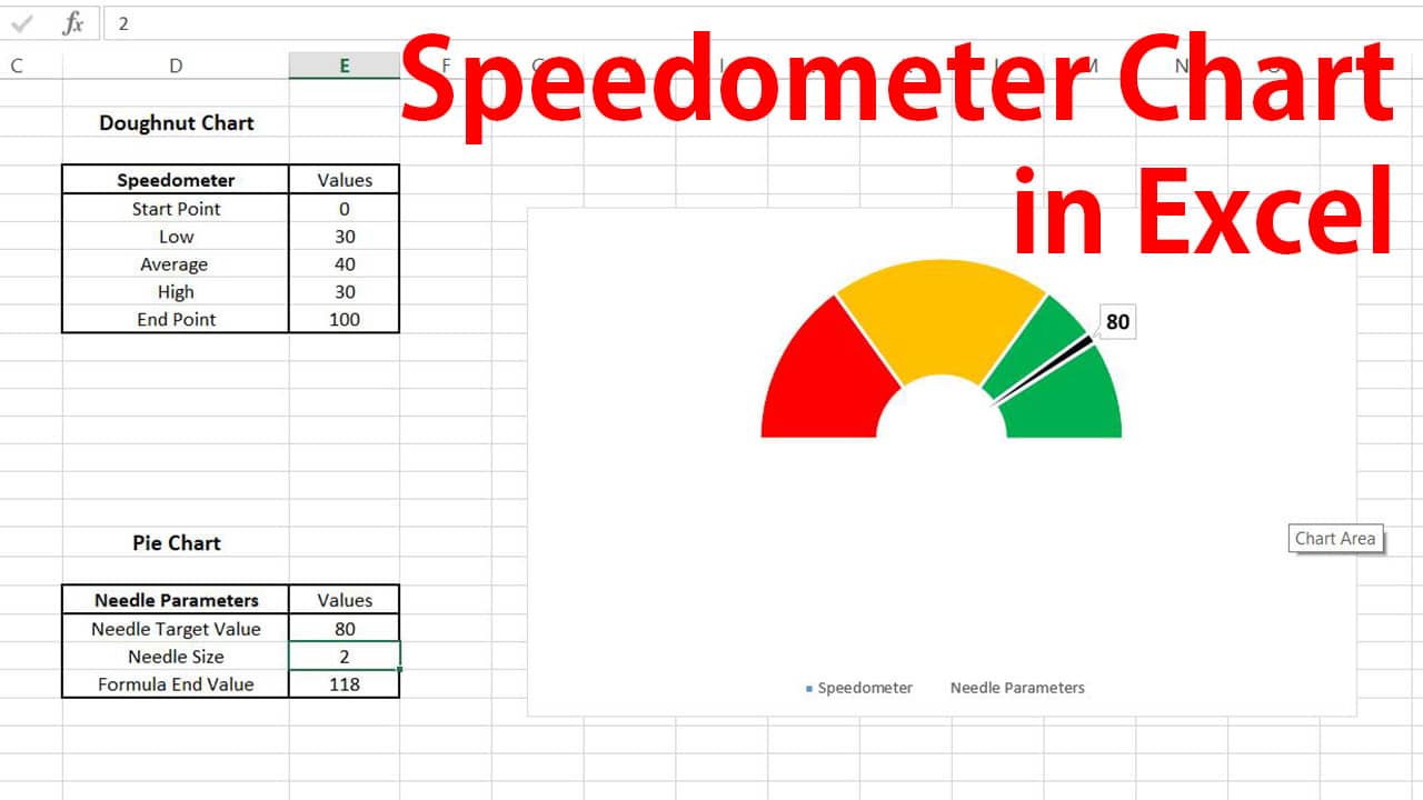
Performance values (Doughnut Chart)
- 0 – 30: Low performance
- 31 – 70: Average performance
- 71 – 100: High Performance
Needle Operators (Pie Chart)
To begin with, let’s consider a random digit for the needle target value as 50 and the size of the needle as 2. The Formula End Value assists in better functionality and operability of the needle and can be computed as below.
Formula End Value = Sum (Values in Parameter table) – (Needle Target Value + Needle Size)
Step 1: Creation of the doughnut chart
Manually input all the values in two different tables on the sheet. To initiate making the first chart, go to the menu bar and insert Doughnut chart. On the screen, do a right-click and say “Select Data”. Then click “Add New” and enter the series name i.e. Speedometer and add all the values in the option provided.


Once present on the screen, we need to customize the diagram for proper structuring to make it appear as a speedometer dial. Select the chart, and from the features available at the right edge of the screen, under the series option, change the angle of the first slice to 270 degrees.
Change the color of the blue component in the circle to No Fill. Similarly, select the individual components in the structure and change their colors as per your choice. One done, the doughnut chart is ready and modified.


Step 2: Creation of the pie chart
With a right-click on the existing chart on the spreadsheet, follow the same guidelines to create another doughnut chart i.e. Select Data >> Add New>> Enter the values from the second table.


Once the second doughnut is created, we have to change its chart type to Pie with a right-click on the screen as shown in the screenshots.


Step 3: Creating Needle
After generating both the charts, we need to format the newly added chart to create the needle. Select the pie, navigate to the series option as before and input the angle of the first slice to 270 degrees as done previously. Select No Fill for all the components except the needle and change the color of the pointer or needle to black.


To magnify the dial of the speedometer, we need to broaden the semicircular colored components by simply selecting the structure and valuing the Doughnut Hole Size to 35%.

Step 4: Adding Data Labels
The final step would be to add data labels for numerical clarity and effectiveness of use. Select the pie chart and do a right-click on the screen and pick “Add Data Labels” and select “Add Data Callouts”


Place the cursor on the data that has popped on the screen, and on the input column provided on the menu bar, enter the cell value of the Needle Target parameter so that the data label number displays 50.

The chart is now ready and to test its functioning, let’s change the value of the pointer to 80 as portrayed below. Once successful, change the target value to any digit to validate the performance quotient of the employee.

To sum up, the speedometer creating procedure in Microsoft Excel, one can conclude that process can project some level of complexity to beginners and laymen in designing as it involves the creation of two charts. But the ease of making and designing the charts with preset dimensions and guidelines through this application makes it a less time consuming and lucrative process.